Build a Dynamic Income Tax Calculator – Part 1 of 2

By David H. Ringstrom, CPA

Look-up formulas are one of Excel’s most powerful features. Instead of manually linking to a worksheet cell, such as =A2, a look-up formula allows you to provide a criteria, such as taxable income, and have the formula automatically return the proper tax rate. This enables you to quickly run through various scenarios with your clients by simply changing the taxable income value. However, income tax calculations in particular can become tricky, as your formula also needs to refer to one of four different tables. In part 1 of this two-part series I’ll explain how to use the VLOOKUP formula to cross-reference tax rates from a single table. I’ll then show you how to use Excel’s INDIRECT function make your VLOOKUP formula refer to the proper table based on your choice of filing status in an adjacent worksheet cell. Next month, in part 2 of this series, I’ll show you how to condense all four tables into one, and use the MATCH and INDEX functions instead of VLOOKUP.

Click here to download the accompanying Income Tax Calculator spreadsheet.

Understand VLOOKUP

As you might infer, VLOOKUP performs vertical look-ups, which means it looks at columnar ranges. A similar function, called HLOOKUP, looks across rows, but for this article I’ll only focus on VLOOKUP.  This is an ideal function to use when you need a formula to return a marginal tax rate, as shown in Figure 1. First, let’s discuss the VLOOKUP function, which has 4 arguments:

• Lookup_Value: The value that you’re searching for within a table. For instance, this might be a contact’s name, a part number, or in Figure 1, an income tax rate.
• Table_Array:  A range of two or more columns that comprises your data. For instance, in Figure 1, the tax brackets are in the first column, the marginal rate in the second column, and the base tax is in the third column.  VLOOKUP always looks for the Lookup_Value in the first column of the table array.
•  Col_Index_Num: The column number within the Table_Array contains the data that you want to return. Using Figure 1 as an example, we’d specify 2 if we want the income tax rate, or 3 for the base tax.

Caution: VLOOKUP will return a #VALUE! error if you enter a number less than 1 for the Col_Index_Num. Further, VLOOKUP will return a #REF! error if you specify a number greater than the number of columns in the Table_Array.

• Range_lookup: This optional argument enables you to specify between an approximate match or exact match:
  • Approximate match:  By default, VLOOKUP returns an approximate match, which means if it can’t find the Lookup_Value in the first column of the Table_Array then it returns the next largest value. You can either omit this argument, or enter TRUE to indicate that an approximate match is acceptable.

Trap: Approximate matches require the first column of the Table_Array be sorted in ascending order —otherwise VLOOKUP may return an incorrect value.

• Exact Match: Specify FALSE for this argument if only an exact match is acceptable. VLOOKUP returns #N/A if it cannot find the Lookup_Value in the first column of the Table_Array.

Caution: VLOOKUP matches on the first instance of the Lookup_Value. Thus, if your value appears more than once in column A, VLOOKUP will only return the first instance.

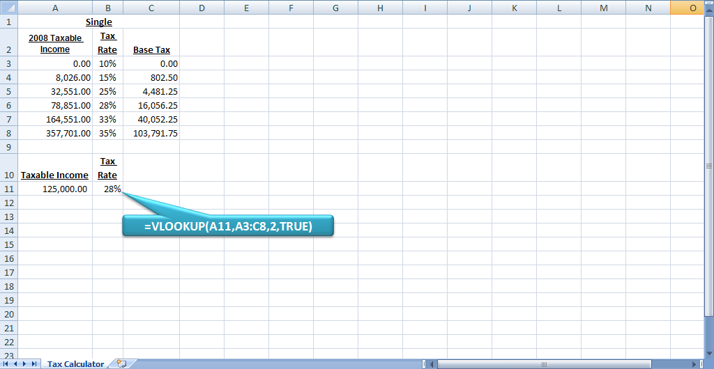Figure 1: We’ll use VLOOKUP to create a simple income tax calculator.

Marginal Tax Rate Look-Up

Now that you understand the inputs for VLOOKUP, let’s walk through an example:

1. Enter the word Single into cell A1 of a blank worksheet.
2. Enter these into cells A2 through C8 of a blank worksheet, as shown in Figure 1:

3. Enter the words Taxable Income in cell A10.
4. Enter the words Tax Rate in cell B10.
5. Enter a taxable income number in cell A11, such as 125,000.
6. Enter this VLOOKUP formula cell B11:

=VLOOKUP(A11,A3:C8,2,TRUE)

                The arguments for the function are as follows:

• A11 represents the Lookup_Value, which returns the taxable income amount
• A3:C8 represents the Table_Array, or the coordinates of the tax table
• 2 represents the Col_Index_Num, which indicates that we want the tax rate from the second column of the table
• True represents the Range_Lookup, which indicates that we want an approximate match, or the closest tax bracket for the taxable income amount.

The formula in cell B11 should return 28% if you entered 125,000 in cell A11.

Shortcut: Since we’re not seeking an exact match, we can omit the Range_Lookup argument and shorten the formula to this:

=VLOOKUP(A11,A3:C8,2)

Conversely, our formula would look like this if we did want an exact match:

=VLOOKUP(A11,A3:C8,2,FALSE)

Tax Calculation

Our formula in cell B11 now determines the marginal tax rate, so now we’ll calculate the tax liability. We can see that income of $125,000 places our taxpayer in the 28% tax bracket. However, 28% doesn’t apply to every dollar of their income — only to income greater than $78,850. We’ll add the base tax of $16,056.25 to this calculated amount, for a total tax of $28,978.25. The formula to perform this calculation is somewhat complex, so we’ll build it in stages:

1. Enter the words Tax Liability in cell C10.
2. Enter this formula in cell C11:

=VLOOKUP(A11,A3:C8,1)

We specify 1 for the Col_Index_Num, so that we can return the starting point of our tax bracket. Based on income of $125,000, the formula should return $78,851.

3. Modify the formula in cell C11 to look like this:

=A10-(VLOOKUP(A11,A3:C8,1)-1)

Your formula should now return $46,150. In this case we’re taking our taxable income of $125,000 from cell A11, subtracting the tax bracket of $78,851, and then subtracting $1 from that amount. This is because our client must pay tax of 28% of all income greater than $78,850.

4. Modify the formula in cell C11 to look like this:

=(A11-(VLOOKUP(A11,A3:C8,1)-1))*B11

Your formula should now return $12,992, which is $46,150 multiplied by 28%.

5. The last step is to add the base tax amount, which requires a second VLOOKUP. Modify the formula in cell C10 to look like this:

=(A11-(VLOOKUP(A11,A3:C8,1)-1))*B11+VLOOKUP(A11,A3:C8,3)

The formula should now return $28,978.25, as shown in Figure 2.

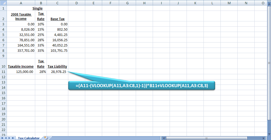Figure 2: The spreadsheet now calculates the tax liability.

Expand the Calculator

Since our formula works with a single table, we’ll now add the three additional tables to the spreadsheet. After that we’ll then assign range names to each table, add a filing status input, and then incorporate the INDIRECT function into our VLOOKUP formulas. Here’s how:

1. Add the remaining three tables, as shown in Figure 3:

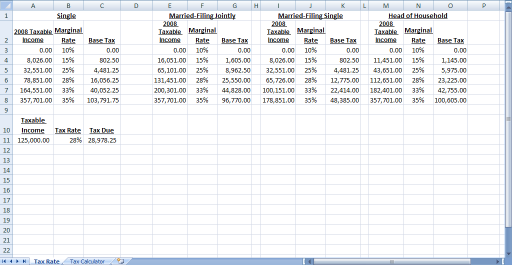Figure 3: Add the additional tables to your spreadsheet.

2. The next step is to assign a range name to each table. This will allow us to refer to each table by name, such as Single, rather than by cell coordinates, such as A3:C8. To do so, select cells A3:C8, and then enter the word Single in the Name Box, as shown in Figure 5.

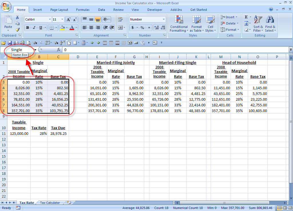Figure 4: You can use the Name Box to assign a range name to a cell or block of cells.

3. Select cells E3:G8, and assign the name MarriedJoint
4. Select cells I3:K8, and assign the name MarriedSingle.
5. Select cells M3:O8, and assign the name HeadOfHousehold.

Name limitations: You cannot use spaces or dashes within range names, nor can you start a range name with a number. Many users use the underscore character in place of spaces, such as Head_of_Household.

1. Enter the words Filing Status in cell D10.
2. Use the Data Validation feature to create an in-cell drop-down list in cell D11:

1. Excel 2007: Choose the Data Validation icon in the Data Tools section of the Data ribbon.

Excel 2003 or earlier: Choose Tools, and then Data Validation.

1. In all versions of Excel, choose List, and then enter this into the Source field, as shown in Figure 5:

Single,MarriedJoint,MarriedSingle,HOH

Caution: Be sure that the contents of the Source field exactly match the range names that you assigned to each of the tables.

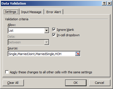
Figure 5: Enter these settings in the Data Validation window.

1. Click OK. At this point, a drop-down list should appear when you click on cell D11, as shown in Figure 6.

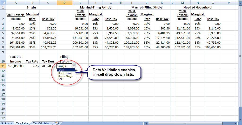
Figure 6: Data Validation provides an in-cell dropdown list.

8. Modify the formula in cell B11 to use the INDIRECT function:

=VLOOKUP(A11,INDIRECT(D11),2)

Tip: You’re simply replacing A3:C8 with INDIRECT(D11).

9. Modify the formula in cell C11 to use the INDIRECT function:

=(A11-(VLOOKUP(A11,INDIRECT(D11),1)-1))*B11+VLOOKUP(A11,INDIRECT(D11),3)

INDIRECT: The INDIRECT function enables you to convert text into an Excel address. In this case, we can use INDIRECT to change between one of four tables without having to modify the formulas in cells B11 and C11.

10. At this point you can test your work by making different choices from the drop-down list in cell D11:

• MarriedJoint should cause cell C11 to return $23,937.50
• MarriedSingle should cause cell C11 to return $30,614.50
• HOH should cause cell C11 to return $26,683.00

You now have a functional tax calculator that we’ll streamline next month in Part 2 of this series.

The views and opinions expressed in this column are those of the author and do not necessarily reflect theopinions of Microsoft.

This article first appeared Microsoft Professional Accountant's Network newsletter.

David H. Ringstrom, CPA heads up Accounting Advisors, Inc., an Atlanta-based software and database consulting firm providing training and consulting services nationwide. Contact David at david@acctadv.com  or follow him on Twitter. David speaks at conferences about Microsoft Excel, and presents webcasts for several CPE providers, including AccountingWEB partner CPE Link