Tag: Excel

Dec 10

Identifying Largest and Smallest Values in an Excel List

Filed under AccountingWEB articles, AccountingWEB Excel articles, Excel

By David Ringstrom, CPA

Periodically, you may wish to rank a series of items within an Excel spreadsheet. Many users often rely on sorting data in ascending or descending order. I'll describe an alternative that uses the LARGE and SMALL functions to create an ordered list of whatever you'd like to rank.

You're probably already familiar with the MIN and MAX functions in Excel, which return the smallest or largest value within a list, respectively. As shown in Figure 1, MIN indicates the smallest value is 191, and the largest value is 958. MIN and MAX are limited to the single smallest or largest values respectively, but LARGE and SMALL allow you to return the second largest or third smallest value if you choose. I'll explain these functions in a moment, but first let's explore MIN and MAX.

Figure 1: MIN and MAX return the largest and smallest values from a list, respectively.

As shown in Figure 1, the MIN and MAX functions are similar in nature to the venerable SUM function, except they return the single smallest or largest value, respectively, instead of adding up values. The SMALL and LARGE functions work in a similar fashion, but with an extra argument:

=SMALL(array,k)

=LARGE(array,k)

In these functions, array is a range of cells, and k is the nth value you wish to return. As shown in Figure 2, =LARGE(B2:B11,2) would return 872 as the second largest value, while =SMALL(B2:B11,3) would return 266 as the third smallest value. By way of comparison, the following formulas would both return 958 and 191 for the largest and smallest values, respectively:

=MIN(B2:B7)

=SMALL(B2:B7,1)

=MAX(B2:B7)

=LARGE(B2:B7,1)

Figure 2: LARGE and SMALL return the nth values from a given list.

If you're creating a list of the top or bottom 10 values, it can be tedious to manually edit each LARGE or SMALL function with the proper value for the k argument. To save time, I use the ROW function, either inside the LARGE or SMALL function or in a separate column. The ROW function returns the row number for a given cell. If you enter this in cell D2, Excel will return 2:

=ROW()

In Figure 3 you can see that I entered this formula in cell D2:

=ROW()-1

In this case, ROW() would return 2 because it's entered on the second row, so subtracting 1 changes the result to 1. Alternatively, I could provide the address of a cell in row 1 of the worksheet:

=ROW(D1)

Figure 3: These formulas are the basis for creating a ranked list without re-sorting the source data

In cell F2, I entered this formula:

=LARGE(B$2: B$11,D2)

Depending upon my needs, I might have used this formula instead:

=LARGE(B$2: B$11,ROW()-1)

The dollar signs in the formula instruct Excel not to change the row numbers when I copy the formula down. The last bit of information that you'll likely want is to associate a name with the values that you've isolated. To do so, you can use the MATCH and INDEX functions together in cell E2:

=INDEX(A$2:A$11,MATCH(F2,B$2:B$11,0))

I'll explain MATCH and INDEX in more detail in an upcoming article, but for now the short answer is that in this case MATCH is determining which row a sales figure amount is on, and then INDEX returns the corresponding text from column A. This is akin to VLOOKUP, but with the flexibility of being able to look up data from the left, which VLOOKUP can't do without making a special provision.

There's one caveat to this approach that you should be aware of. If the same value is on your list twice, then MATCH/INDEX will return the corresponding name twice. Next week I'll describe how you can use the COUNTIF function to create a tiebreaker that will give you a unique value to match for each item in the list.

In any case, once I have the formulas in cells D2 through F2 in place, I'm able to copy the formulas down as many rows as needed without any additional modifications, as shown in Figure 4. Do keep in mind that if you drag too far, LARGE or SMALL will return #NUM!.

Figure 4: If you drag the formulas in cells D2:F2 too far, LARGE will return #NUM!.

A previous version of this article first appeared on www.accountingweb.com .

About the author:

David H. Ringstrom, CPA heads up Accounting Advisors, Inc., an Atlanta-based software and database consulting firm providing training and consulting services nationwide. Contact David at david@acctadv.com or follow him on Twitter. David speaks at conferences about Microsoft Excel, and presents webcasts for several CPE providers, including AccountingWEB partner CPE Link

AccountingWEB, Excel

Jun 22

Automating Chart Titles

Filed under AccountingWEB articles, AccountingWEB Excel articles, Excel

By David Ringstrom

Recently, I described how you can use Excel's Table feature to have charts expand automatically. In this article, I'll show how you can further automate your chart with a self-updating title.

To create a chart in Excel 2007 and later, create a data set like the one shown in cells A1 through E3. Next click on cell A1, choose Insert, Column, and then the first 2-D option, as shown in Figure 1.

Figure 1: Creating a chart from a Table in Excel 2007 and later.

The next step is to add a title to the chart. To do so, click once on the chart to select it, and then choose Layout, Chart Title, and then Above Chart, as shown in Figure 2. To manually change the title, you can click on the title field within the chart and edit the text as desired. However, we can use a formula to make the title dynamic instead.

Figure 2: Adding a title to the chart.

To automate your chart title, use two worksheet functions together:

COUNTA – This worksheet function returns the number of non-blank cells in a given range.
INDEX – This worksheet function returns data from cell coordinates that you provide.

Use COUNTA to determine the number of non-blank cells in row 1. This assumes you won't have any data to the right of your source data, shown in Figure 1. If you've entered four months of data, then COUNTA will return the number 5, because there will be five non-blank cells in the row. You'll then use the INDEX function to return the word “April.” To do so, you'll tell the INDEX function to look across row 1 of your worksheet, and return data from the nth cell, as provided by COUNTA. The formula will take this form:

=INDEX(1:1,COUNTA(1:1))

You may wish to add additional narrative, such as the word “Sales.” To do so, you can use a technique known as concatenation. Although Excel has a CONCATENATE worksheet function, I use this approach instead:

=INDEX(1:1,COUNTA(1:1))&” Sales”

In essence, I use an ampersand to join the additional text to my formula. Such text must be enclosed in double quotes.

The aforementioned formula can be entered in any cell in your worksheet. I've chosen to place it in cell A5, just below my source data, as shown in Figure 3.

Figure 3: A simple formula can return the month of the latest data in your chart.

You're now ready to automate your chart title. To do so, click on the title of your chart, and then click in the Formula bar. Click on the cell that contains your title formula, such as cell A5 in this case, and then press Enter, as shown in Figure 4.

Figure 4: Chart titles can reference a formula in a worksheet cell.

To make the chart completely dynamic, click on cell A1, choose Insert, Table, and then press Enter, as shown in Figure 5. My previous article in this series describes this technique in more detail.

Figure 5: Excel's Table feature automates charts such that new data appears automatically.

Your chart is now dynamic. If you've followed all of the steps in this article, you should be able to add a new column of data for May and see the new data and title automatically, as shown in Figure 6.

Figure 6: New data appears on the finished chart, along with a self-updating title.

Note: There are a couple of caveats to be aware of with regard to automating charts. First, if you make the data into a Table before you create your chart, Excel may group the data. To change this, click the Switch Rows/Columns button on the Design tab. Secondly, when automating chart titles, you must reference a worksheet cell, and your formula reference must include a worksheet name. Thus, you can't click on the title and enter =A5 in the formula bar. You must instead use the form =Sheet1!A5.

Stay tuned, as my next article in this series will explain the technique I use to utilize clip art within charts.

A previous version of this article first appeared on www.accountingweb.com .

About the author:

Excel

Jun 16

Excel Tip: Using Today() versus NOW()

Filed under AccountingWEB articles, AccountingWEB Excel articles, Excel

By David Ringstrom, CPA

Many users rely on the NOW() function to return today's date in a spreadsheet. This is a perfectly valid purpose, but in certain cases NOW() can cause a formula headache.

The NOW() function returns both today's date, but also the current time as well. For instance, if it's 12:00 p.m. on December 21, 2012, the formula =NOW() in a worksheet cell will return 41,264.50. This is because 12/21/12 is 41,264 days subsequent to January 1, 1900.

The .50 portion represents half of a twenty-four-hour day. Thus, if you're comparing a static date value, such as 12/21/12 to the NOW() function, Excel will indicate that they don't match, because 41,264 isn't equal to 41,264.50.

The solution for comparing dates is to use the TODAY() function instead, since it returns the date portion only; for example, 41,264 for 12/21/12.

A previous version of this article first appeared on www.accountingweb.com .

About the author:

Excel, Worksheet Function

Jun 16

Excel Tip: Pasting Text into Excel 2010

Filed under AccountingWEB articles, AccountingWEB Excel articles, Excel

By David Ringstrom, CPA

From time to time, you might copy a list of data in text format from a webpage, report screen, or other source to the Windows clipboard. In such cases, Excel 2010 offers a hidden shortcut that makes it easier to break such data into columns.

With text data on the clipboard, click the lower half of the Paste button on the Home tab, and then choose Use Text Import Wizard.

This feature allows you to parse delimited data into columns based on a separator, such as tab, semicolon, comma, space, or a single character of your choice. Or, you can choose Fixed Width and manually place column breaks where you need them. This saves the step of pasting data into a worksheet column and then manually launching the Text to Columns wizard on the Data tab of the ribbon.

A previous version of this article first appeared on www.accountingweb.com .

About the author:

Excel

Jun 16

Excel Tip: Data Entry Shortcut

Filed under AccountingWEB articles, AccountingWEB Excel articles, Excel

By David Ringstrom, CPA

If you find yourself making repetitive entries into an Excel spreadsheet, press Alt-Down to view a drop-down list of previous entries in the current column.

Arrow down the list and press Enter to make a selection.

Keep in mind that this technique works with text only, not numbers, and your cursor must be in or adjacent to a contiguous block of non-blank cells.

A previous version of this article first appeared on www.accountingweb.com .

About the author:

Excel

Jun 16

Excel Tip: Automatic Backup of Key Excel Workbooks

Filed under AccountingWEB articles, AccountingWEB Excel articles, Excel

By David Ringstrom, CPA

From within the Save As dialog box of Excel, click the Tools menu, and then choose General Options.

Click the checkbox to Always Create Backup to have Excel automatically create an .xlk version of your file. For instance, if you save the workbook as Participant Hours Tracking.xlsx, each time you save the file Excel will create or overwrite a second workbook named Backup of Participant Hours Tracking.xlk.

The backup copy is only as old as the last time that you saved, so if you compulsively save every five minutes, your backup will always be five minutes old, but it does offer a bit of a safety net.

A previous version of this article first appeared on www.accountingweb.com .

About the author:

Excel, Worksheet Function

Jun 14

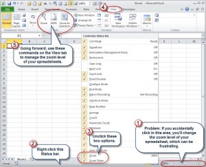
Disabling Excel’s Zoom Slider

Filed under Excel

The Zoom Slider in Excel 2007 and later can be disabled.

Excel

Jun 01

Automating Excel Charts in Two Keystrokes

Filed under AccountingWEB articles, AccountingWEB Excel articles, Excel

By David H. Ringstrom, CPA

Readers of a certain age will remember a television game show in which contestants would state “I can name that tune in five notes,” or some such number of notes. Along those lines, I'll show you how to automate an Excel chart with just two keystrokes. I'll first show you the typical way that most users accomplish adding data to a chart, and then I'll share the simple technique that eliminates this mundane need.

Let's say that you maintain a monthly chart, such as the one in Figure 1, where you periodically add another column of data. In Excel 2007 and 2010, most users carry out these steps to expand the chart:

Figure 1: Most users manually expand charts like this one.

Add a new column of data, such as for June.
Click once on the chart, and then choose Select Data from the Design tab of the ribbon.
As shown in Figure 2, change the Source Data range to be $A$1:$G$3, and then click OK. The month of June should then appear on the chart. Repeat this action month after month.

Figure 2: Steps involved in manually expanding a chart in Excel 2007 and later.

Power user tip: Typically pressing an arrow key within the Source Data field inserts an extraneous cell address. Press F2 to toggle to Edit mode, which means you can use the arrow keys to navigate within the field.

Alternatively, you can let the Select Data button molder. In Excel 2007 and 2010, click any cell within your chart's source data, press Ctrl-T, and then press Enter. Add a new month of data into the worksheet, and you'll see that the chart expands itself automatically, as shown in Figure 3.

Figure 3: Charts based on tables expand automatically.

Ctrl-T is the keyboard shortcut for the Table feature, which first appeared in Excel 2007. It's actually a revamp of the List feature that has long existed on the Data menu of earlier versions of Excel. Charts automatically adopt the dynamic nature of tables, which expand automatically when you add columns or rows of data.

Unfortunately this technique isn't available in Excel 2003 and earlier. The predecessor List feature doesn't interact with charts in the same fashion as the Table feature in Excel 2007 and later. However, if you're using a current version of Excel, you can use this keystroke process to instantly automate your existing charts.

A previous version of this article first appeared on www.accountingweb.com .

About the author:

AccountingWEB, Charts, Excel

Mar 25

You Can’t have a History

Filed under Excel

Did you know that it's not possible to assign the name History to an Excel worksheet? This is a reserved sheet name that Excel uses in conjunction with the rarely used Track Changes feature that appears on the Tools menu. To work around this limitation, add a period or a space after the word History.

Excel, Oddities

Mar 25

Excel Programming Reference Book

Filed under Excel, Recommended Books

Excel Programming Weekend Crash Course is a great reference book for anyone interested in learning how to create macros in Excel. Even experienced VBA users will pick up a few new tricks. The material is broken down into chapters that take 30 minutes to complete, so it's easy to work through the material at your own pace.

Although this book was published in 2003, Excel programming hasn't changed much over the years, so this is still a relevant reference guide even for Excel 2010 and beyond.